金融数据中的时间序列分析——ARMA模型

鱼籽酱

在对金融数据进行分析时，不可避免地会遇到时间序列数据，常见的时间序列模型有AR自回归模型，MA移动平均模型和 ARMA 模型等模型。本文主要介绍 ARMA 模型 ^[1] 。

ARMA 模型可以理解为 AR(p) 自回归模型和 MA(q) 移动平均模型的合并

AR(p) 模型尝试解释我们在交易市场中观察到的动量和均值回归效应
MA(q) 模型则试图捕获白噪声项的冲击效应

ARMA 作为二者合并的金融时间序列模型，既可以捕获动量、均值回归效应，也能够捕获冲击效应。同时 ARMA 模型不考虑波动集群现象——收益率的巨大变化通常伴随着进一步的巨大变化。

ARMA(1,1) 模型可以表示如下：

e(t) 代表白噪声，且相应的期望为0（ E[e(t)] = 0 ）

ARMA 在使用时候通常比单独使用 AR(p) 自回归模型或 MA(q) 模型需要更少的参数。

下面根据给定的参数模拟一个 ARMA(2,2) 的过程，然后根据模拟的数据拟合一个 ARMA(2,2) 模型，来看看它是否能够正确地估计那些参数。这里设置自回归参数 α 为[0.5,-0.25]，移动平均参数 β 为[0.5,-0.3]

首先导入相应的包

 import pandas as pd
 import numpy as np
 import statsmodels.tsa.api as smt
 import statsmodels.api as sm
 import scipy.stats as scs
 import statsmodels.stats as sms
 import matplotlib.pyplot as plt
 %matplotlib inline

然后编写对应的函数

 def tsplot(y, lags=None, figsize=(10, 8), style='bmh'):
     if not isinstance(y, pd.Series):
         y = pd.Series(y)
     with plt.style.context(style):    
         fig = plt.figure(figsize=figsize)
         layout = (3, 2)
         ts_ax = plt.subplot2grid(layout, (0, 0), colspan=2)
         acf_ax = plt.subplot2grid(layout, (1, 0))
         pacf_ax = plt.subplot2grid(layout, (1, 1))
         qq_ax = plt.subplot2grid(layout, (2, 0))
         pp_ax = plt.subplot2grid(layout, (2, 1))
         y.plot(ax=ts_ax)
         ts_ax.set_title('Time Series Analysis Plots')
         smt.graphics.plot_acf(y, lags=lags, ax=acf_ax, alpha=0.05)
         smt.graphics.plot_pacf(y, lags=lags, ax=pacf_ax, alpha=0.05)
         sm.qqplot(y, line='s', ax=qq_ax)
         qq_ax.set_title('QQ Plot')        
         scs.probplot(y, sparams=(y.mean(), y.std()), plot=pp_ax)
         plt.tight_layout()
     return

下面模拟生成对应的数据

 max_lag = 30
 n = int(5000) # 总的样本个数
 burn




    
 = int(n/10) # 拟合前丢弃的样本量
 alphas = np.array([0.5, -0.25])
 betas = np.array([0.5, -0.3])
 ar = np.r_[1, -alphas]
 ma = np.r_[1, betas]
 arma22 = smt.arma_generate_sample(ar=ar, ma=ma, nsample=n, burnin=burn)
 _ = tsplot(arma22, lags=max_lag)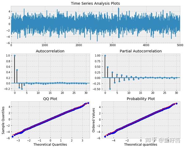

下面对模拟生成的数据拟合 ARMA 模型

 mdl = smt.ARMA(arma22, order=(2, 2)).fit(
     maxlag=max_lag, method='mle', trend='nc', burnin=burn)
 print(mdl.summary())
 ARMA Model Results                              
 ====================================================================
 Dep. Variable:              y   No. Observations:         5000
 Model:             ARMA(2, 2)   Log Likelihood       -7054.211
 Method:                   mle   S.D. of innovations      0.992
 Date:         Mon, 8 Jun 2020   AIC                  14118.423
 Time:                21:27:58   BIC                  14151.009
 Sample:                     0   HQIC                 14129.844
 ====================================================================
                coef  std err        z    P>|z|    [0.025      0.975]
 --------------------------------------------------------------------
 ar.L1.y      0.5476    0.058    9.447    0.000     0.434       0.661
 ar.L2.y     -0.2566    0.015  -17.288    0.000    -0.286      -0.228
 ma.L1.y      0.4548    0.060    7.622    0.000     0.338       0.572
 ma.L2.y     -0.3432    0.055   -6.284    0.000    -0.450      -0.236
                                     Roots                                    
 ====================================================================
                Real         Imaginary         Modulus      Frequency
 --------------------------------------------------------------------
 AR.1          1.0668         -1.6609j          1.9740        -0.1591
 AR.2          1.0668         +1.6609j          1.9740         0.1591
 MA.1         -1.1685         +0.0000j          1.1685         0.5000
 MA.2          2.4939         +0.0000j          2.4939         0.0000
 --------------------------------------------------------------------

如果你运行几次上方的代码，你会发现有些实际的参数值并不在估计的参数的置信区间内。这意味着即使我们知道真实的参数值，在尝试进行模型拟合时也可能会出问题。

然而，出于交易使用的目的，大多时候只要求模型有超过随机预测的结果同时能够产生产生净收益的预测能力，保证长远来看是盈利的。

那在进行模型拟合时，如何决定 ARMA 模型的 p 、 q 这两个值呢？

通常情况下，利用AIC准则去判断一组 (p,q) 参数组合的好坏，同时运用 Ljung-Box test 去判断数据是否被较好地拟合。如果对应的p值大于设定的显著性水平，则可以认为残差是独立的，且是白噪声。

以 ARMA(3,2) 模型为例进行演示

 max_lag = 30
 n = int(5000)
 burn = 2000
 alphas = np.array([0.5, -0.4, 0.25])
 betas = np.array([0.5, -0.3])
 ar = np.r_[1, -alphas]
 ma = np.r_[1, betas]
 arma32 = smt.arma_generate_sample(ar=ar, ma=ma, nsample=n, burnin=burn)
 _ = tsplot(arma32, lags=max_lag)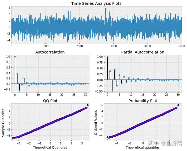

 best_aic = np.inf 
 best_order = None
 best_mdl = None
 rng = range(5)
 for i in rng:
     for j in rng:
         try:
             tmp_mdl = smt.ARMA(arma32,
                       order=(i, j)).fit(method='mle', trend='nc')
             tmp_aic = tmp_mdl.aic
             if tmp_aic < best_aic:
                 best_aic = tmp_aic
                 best_order = (i, j)
                 best_mdl = tmp_mdl
         except: continue
 print('aic: %6.2f | order: %s'%(best_aic, best_order))

得到的 best_order 为（3，2）， best_aic 为14110.88

再进行后续的检验

 sms.diagnostic.acorr_ljungbox(best_mdl.resid, lags=[20], boxpierce=False)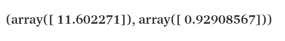

这里的p值大于0.05，说明 ARMA(3,2) 模型能够较好地拟合原始数据。

下面检查一下模型的残差是否是白噪声

 _ = tsplot(best_mdl.resid, lags=max_lag)
 from statsmodels.stats.stattools import jarque_bera