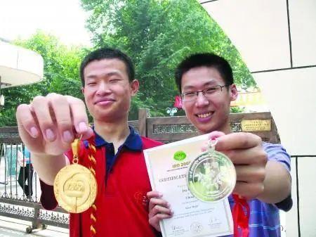
任性的菠菜 · Python - ...· 3 月前 · |
开朗的滑板 · Python3和pyqt5实现控件数据动态显 ...· 5 月前 · |
胡子拉碴的刺猬 · Could not resolve all ...· 5 月前 · |
健身的咖啡豆 · js获取数组第二个元素 - OSCHINA ...· 1 年前 · |
乖乖的小摩托 · nginx架构分析之 事件驱动模型 - ...· 1 年前 · |
腼腆的炒粉
6 月前 |
It was first proven in [ 43 ] that actual network traffic exhibits self-similarity. This work provided the motivation for numerous studies that demonstrated the significant impact of self-similarity on TCP transmissions [ 44 ], or to confirm its occurrence in Wide Area Networks (WANs) [ 45 ]. Self-similarity results in performance degradations, such as mean queue length enlargement and the increase in packet loss probability [ 42 ]. The topic of self-similarity is still relevant in the literature and found its application in e.g., DoS attack detection (e.g., [ 46 ]). Our previous works were also related to this topic. They regarded determining the degree of traffic self-similarity expressed by the Hurst parameter and also using data obtained from the IITiS data traffic traces to examine self-similar properties [ 25 ]. Self-similarity significantly impacts queue occupancy and transmission performance [ 47 ]. For that reason, the samples generated for the purpose of this article are characterized by different degrees of self-similarity.
Artificial Neural Networks have found application in many different domains, e.g., image classification, natural language processing, signal processing etc. Additionally, Deep Learning approaches have become a solution to many problems due to their better ability to extract patterns than shallow learning [ 48 ]. The versatility of neural networks has resulted in them also being frequently used in the network traffic domain for tasks including attack detection [ 49 , 50 ], traffic generation [ 51 ] and classification of the traffic type [ 52 ].
Network traffic and its features are often represented as a time series. To process time-series data with Artificial Neural Networks, different types of networks (e.g., Autoencoders) and layers can be used, namely Recurrent layers (including Long-Short Term Memory (LSTM) layers and Gated Recurrent Unit (GRU) Layers) and 1D Convolutional Neural Networks.
Autoencoders can be built using different types of layers, e.g., Dense Layers or Convolutional layers. The goal of this type of network is to compress input data and then reconstruct it on output [ 53 ]. It can be used for the purpose of data denoising, but also anomaly detection. When the neural network is not able to reconstruct the input data well, it suggests that the sample can be anomalous [ 53 ].
LSTM layers are often used for the purpose of time-series data processing. Single LSTM units solve the gradient vanishing and exploding issues typical for simple Recurrent Layers and are able to propagate gradients over a long period of time [ 54 ]. The key characteristic of this type of layer is that they store the internal state, which enables them to ’remember’ the past information [ 52 ]. Due to that their internal ’memory’ is longer than in the traditional recurrent units.
The alternative for LSTM layers is a GRU layer. It is very similar to LSTM layer, also stores the Long-Time memory of the past information, which is vital for time-series processing. Nevertheless, it is simpler to implement and compute than the LSTM layer, thus more efficient [ 55 ].
Additionally, convolutional layers can be used to process time-series data. In this case, time has to be treated as a spatial dimension [ 22 ]. In fact, it is an efficient alternative to recurrent layers. In a Convolutional Neural Network, transformed time-series data are processed in turns using convolutional and pooling layers. As a result deep, more abstract representations are generated on the basis of raw data. Processing ends with a classifier part (Multi-Layer Perceptron), which consists of dense layers.
In this paper, we used artificial neural network models to develop an active queue management mechanism. The neural networks were trained to mimic the operation of the AQM based on the fractional order controller mechanism. The training data were generated based on simulation data, and a detailed description of the learning model is given in this section.
The neural network model was based on four convolutional layers and two dense layers. After each convolutional layer, the data were normalized and the results were averaged. Additionally, a dropout layer was placed to prevent over-fitting to the learning data. Python and Keras libraries were used to implement the model. The conceptual structure of the model used in this paper is presented in Figure 1 . To design this model structure we relied on the experience of our earlier work [ 25 ], where the degree of self-similarity of network traffic was classified using Convolutional Neural Networks expressed by Hurst parameter.
In order to prepare the training set for the proposed neural network model, network simulations were performed, reflecting the queueing behavior of a fractional order controller . The values of the fractional order controller parameters have been presented in the Table 1 . These values were determined based on our previous work [ 26 ]. The results of these articles have shown that the choice of controller parameters significantly affects the queue length control properties. The process of choosing proper AQM/PI controller parameters is non-trivial. It has a significant impact on the packet dropping function (i.e., for an integral order it can strengthen and accelerate the response of a controller). Properly selected AQM parameters should allow us to obtain adaptation to the changing transmission conditions and desired queue behavior. We discussed the influence of these parameters on queue behavior in papers [ 15 ]. The controller parameters were chosen in such a manner that controller was the weakest controller, and controller was the strongest one, which implies a large number of packet rejections and ease of maintaining the desired queue length.
To obtain training data for an AQM model based on Convolutional Networks, network simulations were performed using the AQM mechanism. For this purpose, the discrete event simulator SimPy (written in Python) was used. This software is available under the MIT License and has been used in our previous works regarding the evaluation of AQMs [ 21 , 26 ].
Our simulation model was a discrete model of a queue. The simulation time was divided into discrete time intervals of length . Arrival of a packet was generated (or not) in a given time slot by a traffic source. The source of traffic was self-similar and based on Fractional Gaussian Noise (FGN) process. The advantages of such a source have been described previously in the articles [ 10 , 15 , 25 ].
All experiments considered different degrees of traffic self-similarity expressed using Hurst parameter. In experiments the Hurst parameter changed between (no correlation) and (high degree of LRD).
The input intensity coefficient was set to a constant value . Thus, the simulation packet source always had a constant intensity. Parameter represents the time of packet processing and dispatching (probability of taking a packet from the queue). Different values of this coefficient were used in the experiments. The parameter took values between (moderately stressed system) to (highly stressed system). This choice of simulation parameters allowed us to observe all properties of the AQM mechanism.
In our experiments, we considered different numbers of items from queue occupancy history taken into consideration in the samples used to train Convolutional Networks. For simplicity, we refer to this number of samples as ’CNN History’. This length corresponded to the number of time slots in the simulation model that were used as training data for the network. For example refers to time intervals taken into consideration. Throughout this time, we observed the behavior of the AQM queue.
Thus, the training data consisted of:
where .
Decision Class | Probability Interval [%] |
---|---|
1 | [0;5) |
2 | [5;15) |
3 | [15;25) |
4 | [25;35) |
5 | [35;45) |
6 | [45;55) |
7 | [55;65) |
8 | [65;75) |
9 | [75;85) |
10 | [85;95) |
11 | [95;100] |
Therefore, we considered different lengths of queue occupancy history, because from the perspective of the router, which is a low resource device, minimizing the length of the history would be beneficial. In our study, we tried to determine the minimum acceptable length of n last items of the queue’s occupancy history.
For each probability interval, one million one-dimensional learning records were prepared. Therefore, the training set consisted of 11 million records. They contained transmission information such as the length of the queue in each consecutive time slot, the number of dropped packets, and the value of the controller’s packet rejection probability function. We present the process of data preparation in Figure 2 . This amount of data seemed to be sufficient in comparison with the cardinality of data reported in the literature [ 56 ].
Input data prepared in such a manner were used in the process of supervised learning of the neural network models. In order to train the model and minimize the cost function, the optimizer Adaptive Moment Estimation (Adam) was used with the following parameters:
where: is the learning rate, is the exponential decay rate for the first moment estimates and is the exponential decay rate for the second moment estimates. The Adam optimizer is expressed by the equation [ 57 ]:
where v is the first moment, which resembles momentum that records the past normalized gradient, s is the second moment and g denotes the gradient descent.
In both the four convolutional layers and the two dense layers, ReLU was used as the activation function and Sigmoid/Softmax functions were used to determine the activation of the output layer. Categorical cross-entropy was used as a cost function. Figure 1 shows the conceptual structure of a neural network model used for the purpose of active queue management mechanism.
We limited the training process to 10 epochs. This value was sufficient, since the values start to stabilize after only 5–6 epochs, as confirmed by the results in Table 3 , Table 4 and Table 5 . We also compare the accuracy of the model, when Softmax activation function ( Table 3 ) and Sigmoid activation function ( Table 4 ) were used in the output layer. Higher results were obtained for the Sigmoid function.
Softmax | ||||||||
---|---|---|---|---|---|---|---|---|
n History Length | ||||||||
20 | 100 | 200 | 300 | 400 | 500 | 1000 | ||
CNN by behavior | 5 epochs | 52.27 | 54.48 | 54.50 | 56.67 | 58.40 | 58.81 | 51.59 |
6 epochs | 52.36 | 54.88 | 54.68 | 56.70 | 58.42 | 58.84 | 51.72 | |
10 epochs | 52.40 | 55.50 | 54.83 | 56.74 | 58.47 | 58.90 | 51.82 | |
CNN by behavior | 5 epochs | 48.37 | 47.23 | 40.29 | 41.99 | 43.68 | 44.06 | 43.94 |
6 epochs | 48.45 | 47.61 | 40.32 | 42.06 | 43.74 | 44.06 | 44.00 | |
10 epochs | 48.54 | 48.42 | 40.31 | 42.30 | 43.78 | 44.24 | 44.04 | |
CNN by behavior | 5 epochs | 47.07 | 41.83 | 33.80 | 32.30 | 32.92 | 33.79 | 38.45 |
6 epochs | 47.18 | 42.09 | 33.81 | 32.31 | 32.93 | 33.82 | 38.44 | |
10 epochs | 47.41 | 42.62 | 34.18 | 32.32 | 32.92 | 33.83 | 38.50 |
Sigmoid | ||||||||
---|---|---|---|---|---|---|---|---|
n Last Items in Queue Occupancy History | ||||||||
20 | 100 | 200 | 300 | 400 | 500 | 1000 | ||
CNN by behavior | 5 epochs | 55.98 | 73.95 | 80.76 | 83.67 | 85.22 | 86.15 | 88.46 |
6 epochs | 56.04 | 74.06 | 80.88 | 83.80 | 85.39 | 86.31 | 88.74 | |
10 epochs | 56.16 | 74.38 | 81.19 | 84.13 | 85.69 | 86.64 | 89.46 | |
CNN by behavior | 5 epochs | 50.34 | 70.70 | 75.94 | 76.92 | 77.03 | 77.20 | 83.71 |
6 epochs | 50.38 | 70.83 | 76.08 | 77.06 | 77.18 | 77.32 | 84.04 | |
10 epochs | 50.53 | 71.13 | 76.40 | 77.36 | 77.57 | 77.79 | 84.81 | |
CNN by behavior | 5 epochs | 48.77 | 67.16 | 67.54 | 65.65 | 64.39 | 64.04 | 77.46 |
6 epochs | 48.82 | 67.29 | 67.70 | 65.83 | 64.57 | 64.24 | 77.76 | |
10 epochs | 49.06 | 67.60 | 68.03 | 66.23 | 64.99 | 64.68 | 78.68 |
Sigmoid | ||||||||
---|---|---|---|---|---|---|---|---|
n Last Items in Queue Occupancy History | ||||||||
20 | 100 | 200 | 300 | 400 | 500 | 1000 | ||
CNN by behavior 3 | 5 epochs | 49.52 | 67.03 | 68.55 | 68.48 | 68.40 | 68.42 | 70.98 |
6 epochs | 49.58 | 67.12 | 67.70 | 68.65 | 68.60 | 68.61 | 71.30 | |
10 epochs | 49.74 | 67.34 | 68.99 | 69.03 | 69.15 | 69.21 | 72.10 |
In the case of Softmax function ( Table 3 ), the minimum accuracy was 32.3%, and the maximum 58.9%. For the models in which we applied the Sigmoid activation function for the last layer the minimum accuracy was 48.77% (for the network trained on the data from the controller, where the CNN History ), and the maximum 89.46% (for the network trained on the data from the controller, where the CNN History ). Taking all the results into consideration, the best results were obtained for the CNN History , and the worst for the CNN History ( Table 4 ).
In the case of the model trained on data representing the behavior of three controllers simultaneously and the use of the Sigmoid activation function of the output layer, the maximum accuracy was 72.1% for the CNN History (see Table 5 ).
This section presents the behavior of the trained neural network (as assumed in Section 4 and evaluates its effectiveness as an AQM mechanism. This evaluation was performed using previously described simulation mechanisms. During the study, we evaluated the number of packets dropped from the queue and the average queue occupancy. We compared the effectiveness of the neural network-based AQM mechanism with the results of the controller-based AQM mechanism. We used the network traffic with different degrees of self-similarity during the experiments.
To increase the readability of the paper, we present only two extreme cases - the results obtained for a non-self-similar traffic ( ) and for a traffic with high degree of LRD ( ).
The intensity of the packet source in the simulation was assumed to be ( ). On the other hand, the packet service time in a system was set to a constant value ( ) in order to obtain a heavily loaded system.
In our experiments, we evaluated four separate neural network models. The first three neural networks were trained with the data obtained from controllers , , and . The fourth model was trained with data regarding all of these controllers. In the first phase of the experiment, we considered two neural network models (see Figure 1 ): the first one with Softmax, and the second one with Sigmoid activation function of the last layer.
A comparison of Table 3 and Table 4 shows that although Softmax function is more commonly used in the literature as an activation function of the output layer of the neural network for multiclass classification, Sigmoid function performs better in our case. In the worst case, in which the network obtained accuracy of 32.31%, changing the activation function to Sigmoid resulted in significant accuracy increase (65.65%). Additionally, in the best obtained case accuracy changed from 58.90% to 86.65%. Figure 3 and Figure 4 show average queue lengths for AQM mechanism based on neural network. Detailed results are compared on Table 6 and Table 7 for Sigmoid function and on Table 8 and Table 9 for Softmax function. Both presented networks imitate the behavior of the first controller— (see Table 1 ). Comparing the number of discarded packets and the average queue sizes, we find that they are similar regardless of the chosen network activation function in the last layer. As Hurst increases, the number of dropped packets decreases slightly in the case of Sigmoid function (<1%).
AQM | Packet Dropped | Average Queue Length |
---|---|---|
249,878 | 168.98 | |
CNN History = 20 | 251,198 | 172.97 |
CNN History = 100 | 248,936 | 176.45 |
CNN History = 200 | 250,063 | 175.69 |
CNN History = 300 | 249,510 | 166.87 |
CNN History = 400 | 250,104 | 166.23 |
CNN History = 500 | 250,800 | 174.31 |
CNN History = 1000 | 249,561 | 173.33 |
AQM | Packet Dropped | Average Queue Length |
---|---|---|
263,387 | 139.16 | |
CNN History = 20 | 261,678 | 145.66 |
CNN History = 100 | 262,304 | 145.81 |
CNN History = 200 | 262,518 | 147.22 |
CNN History = 300 | 262,935 | 139.28 |
CNN History = 400 | 263,872 | 140.89 |
CNN History = 500 | 263,440 | 142.22 |
CNN History = 1000 | 263,654 | 143.14 |
AQM | Packet Dropped | Average Queue Length |
---|---|---|
249,878 | 168.98 | |
CNN History = 100 | 250,038 | 182.21 |
CNN History = 300 | 250,455 | 164.06 |
CNN History = 500 | 250,017 | 174.73 |
AQM | Packet Dropped | Average Queue Length |
---|---|---|
263,387 | 139.16 | |
CNN History = 100 | 261,271 | 148.89 |
CNN History = 300 | 263,609 | 134.64 |
CNN History = 500 | 264,569 | 145.64 |
Taking into consideration higher accuracy obtained using Sigmoid function, we chose this function to be used in further experiments.
Figure 3 compares the behavior of two AQM mechanisms: controller and the CNN-based AQM trained on the data reflecting the behavior of this controller.
For the CNN model, different lengths of the last n elements of the queue occupancy history (input to the neural network) were considered. Regardless of the value of n , the resulting queue length distributions are similar to the queue length distribution of the controller. For Poisson traffic (non-self-similar traffic, ), the average queue length oscillates between 166 and 176 packets (see Table 6 ). For highly self-similar traffic (parameter ), the average queue length was between 139 and 147 (see Table 7 ). In this case, all the Convolutional Neural Network models (with different numbers of CNN History) obtained larger values of the average queue length, with fewer packets dropped, than the mechanism.
Figure 5 presents the results for stronger AQM mechanism . The detailed results of dropped packets numbers and queue lengths are presented in Table 10 and Table 11 . Because of the fact that the controller was stronger than the one presented above, the obtained average queue lengths were smaller.
AQM | Packet Dropped | Average Queue Length |
---|---|---|
250,314 | 134.72 | |
CNN History = 20 | 249,610 | 135.27 |
CNN History = 100 | 250,657 | 140.37 |
CNN History = 200 | 249,633 | 137.95 |
CNN History = 300 | 249,752 | 142.29 |
CNN History = 400 | 248,852 | 134.86 |
CNN History = 500 | 249,960 | 138.85 |
CNN History = 1000 | 249,744 | 129.60 |
AQM | Packet Dropped | Average Queue Length |
---|---|---|
264,819 | 109.37 | |
CNN History = 20 | 263,014 | 117.57 |
CNN History = 100 | 264,135 | 112.98 |
CNN History = 200 | 264,217 | 115.69 |
CNN History = 300 | 264,668 | 116.24 |
CNN History = 400 | 265,538 | 110.05 |
CNN History = 500 | 264,533 | 112.47 |
CNN History = 1000 | 265,839 | 105.25 |
Figure 6 compares the last pair of controllers: controller , with the corresponding models based on Convolutional Neural Networks. The results prove that this controller is the strongest one. The AQM mechanism increased considerably the number of dropped packets and decreased the obtained queue lengths. In the case of traffic without LRD (see Table 12 , for parameter ) the average queue occupancy oscillateds between 116 and 139 packets, and in the case of traffic characterized by a high degree of LRD (see Table 13 , for parameter ) between 94 and 121 packets.
AQM | Packet Dropped | Average Queue Length |
---|---|---|
250,840 | 117.53 | |
CNN History = 20 | 251,892 | 139.26 |
CNN History = 100 | 250,362 | 136.35 |
CNN History = 200 | 248,878 | 117.67 |
CNN History = 300 | 250,533 | 116.40 |
CNN History = 400 | 250,011 | 118.85 |
CNN History = 500 | 250,166 | 118.67 |
CNN History = 1000 | 249,801 | 118.20 |
AQM | Packet Dropped | Average Queue Length |
---|---|---|
265,707 | 95.13 | |
CNN History = 20 | 265,737 | 121.19 |
CNN History = 100 | 263,952 | 110.79 |
CNN History = 200 | 265,383 | 97.28 |
CNN History = 300 | 266,295 | 94.09 |
CNN History = 400 | 266,366 | 95.79 |
CNN History = 500 | 265,592 | 97.31 |
CNN History = 1000 | 266,184 | 96.90 |
It should be noted that for all three CNN-based AQM models, a more efficient AQM model was obtained compared to the controllers that were used to create the test data. Even for the model that obtained the smallest accuracy during the learning process (48.77%, see Table 4 ), based on non-integer controller data of order , for CNN History , the obtained average queue length was larger than for the base mechanism . This situation occurred both for traffic without LRD (see Table 12 ) and for traffic characterized by a high degree of LRD (see Table 13 ).
In the next simulation step, we evaluated the AQM-CNN mechanism whose learning data were generated from the behavior of all three controllers. Figure 7 shows the queue distribution, and Figure 8 shows the changes in queue occupancy over time. Details of the number of packets dropped and the resulting average queue occupancy are presented in Table 14 for the traffic without LRD and in Table 15 , for traffic with a high degree of LRD.
AQM | Packet Dropped | Average Queue Length |
---|---|---|
CNN 3 History = 20 | 249,727 | 128.75 |
CNN 3 History = 100 | 249,988 | 174.64 |
CNN 3 History = 200 | 250,583 | 164.87 |
CNN 3 History = 300 | 249,907 | 169.98 |
CNN 3 History = 400 | 249,593 | 173.41 |
CNN 3 History = 500 | 250,157 | 138.08 |
CNN 3 History = 1000 | 249,334 | 170.46 |
AQM | Packet Dropped | Average Queue Length |
---|---|---|
CNN 3 History = 20 | 262,841 | 120.94 |
CNN 3 History = 100 | 263,859 | 152.15 |
CNN 3 History = 200 | 262,298 | 137.21 |
CNN 3 History = 300 | 263,205 | 131.49 |
CNN 3 History = 400 | 263,818 | 129.81 |
CNN 3 History = 500 | 263,872 | 127.37 |
CNN 3 History = 1000 | 263,554 | 138.32 |
The results show that when the number of last n elements of queue occupancy history taken as a CNN input is too small (CNN History ), then, independent of the degree of self-similarity of the traffic, the number of dropped packets, and the average queue length, approximates the results obtained using the sets of controllers and (see Table 10 , Table 11 , Table 12 and Table 13 ).
On the other hand, when the considered number of last n queue occupancy history elements is larger (CNN History ), the obtained average queue length increases by 46 packets for traffic without LRD ( Table 14 , for ), or by 32 packets, for traffic characterized by a high degree of LRD (see Table 15 , for ). This means that the resulting queue distribution matches the one of the original and the most efficient controller ( Figure 3 ).
This feature indicates that for the AQM model based on Convolutional Networks, as the number of story elements used increases, the ability of the mechanism to adapt to current Internet transmission conditions also improves.
The paper presents a new Active Queue Management mechanism based on Convolutional Neural Networks and supervised learning.
To train the Convolutional Networks used in the experiments, data obtained through simulation have been used. The training data of the CNN model reflect the behavior of the AQM mechanism, based on a fractional order controller .
In our experiments, we took into account the effect of the degree of traffic self-similarity and long-term dependence on the performance of the proposed mechanism.
We also considered the effect of the number of last n elements of the queue occupancy history, used as input of the neural network, on the efficiency of the proposed mechanism. The best results were obtained for CNN History = 500. The minimum length of CNN History for which results are still acceptable is 100.
In the experiments, neural networks with different number of convolutional layers and different optimizers and cost functions were considered to build the AQM model. After comparing the results obtained with different activation functions, the results have shown that the most efficient model used Sigmoid activation function in the output layer, therefore we chose this function for further experiments. The decisions made in this work were also influenced by our previous work regarding traffic classification in terms of the degree of self-similarity [ 25 ].
The most efficient AQM obtained in our study was based on the Convolutional Neural Network model, trained using the data reflecting the behavior of all three controllers jointly.
The results confirmed that the model based on Convolutional Neural Networks can effectively reproduce the results of the classical AQM algorithm and effectively manage the data transmission. Such a model maintains the assumed average number of packets in the queue and reduces the total number of dropped packets, independent of the degree of traffic self-similarity.
It seems that the proposed mechanism exhibits some advantages over previously proposed mechanisms encountered in the literature. Our previous study [ 26 ] demonstrated that the reinforcement learning methods are well suited for maintaining the assumed queue size. However, in computer networks, the process of controlling packet traffic is more complex. The objective is to maximize the transmission efficiency. This efficiency is characterized by: throughput, delay, and possible retransmissions. Efficiency of AQM mechanisms is influenced by self-similarity of network traffic. The higher the Hurst parameter value is, the greater problems with correct packet management occur. The proposed solution addresses this problem much more effectively. The biggest disadvantage of this solution is greater computational and memory complexity of solutions based on Convolutional Neural Networks. This complexity may affect the difficulty of implementing this solution in real routers.
In our previous study [ 58 ], we used a Linux-based computer as a router. In that study, we used a special router implementation based on a special forwarding mechanism (based on the iptables mechanism), which delivered all packets to the user program implementing AQM. This solution greatly simplifies the research model. Unfortunately, the tests have shown that forwarding packets from kernel space to userspace requires a significant amount of time and is not optimal. In the target solutions the whole implementation should be realized in the kernel of the system. The implementation may be a great challenge on routers with low hardware resources. In such solutions instead of multiplication operations bit shifting is used, which causes calculation errors. For CNN calculations these errors may be too high. However, it seems that the computational power of routers will increase in the future. We want to devote a separate article to the problems of implementing AQMs in real routers.
Conceptualization, J.S. and A.D.; methodology, J.S.; software, J.S.; investigation, A.D., J.S. and S.M.; validation, J.D., D.M.; project administration, J.S.; formal analysis, J.D. and K.F.; data curation, J.S. and D.M.; funding acquisition, J.S.; writing—original draft preparation, J.S., J.D., A.D. and K.F.; writing—review and editing, J.S., J.D.; visualization, J.S., D.M. and S.M.; supervision, A.D. All authors have read and agreed to the published version of the manuscript.
Publication supported by Own Schoolarship Fund of the Silesian University of Technology in year 2019/2020, grant number: 22/FSW18/0003-03/2019.
Not applicable.
Not applicable.
Not applicable.
The authors declare no conflict of interest.
Publisher’s Note: MDPI stays neutral with regard to jurisdictional claims in published maps and institutional affiliations.